无监督学习
本周课程开始进入无监督学习。
一个重要应用是聚类问题:
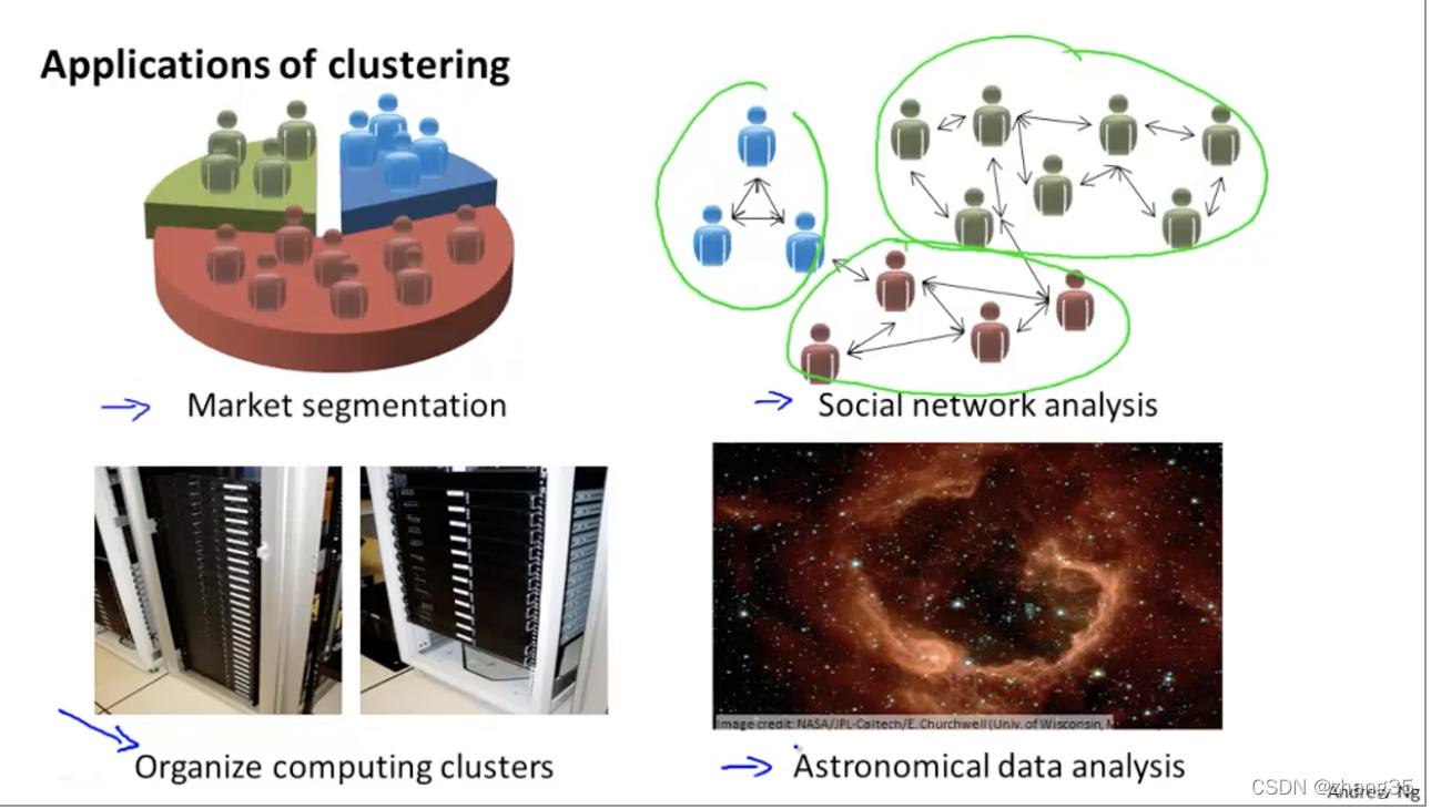
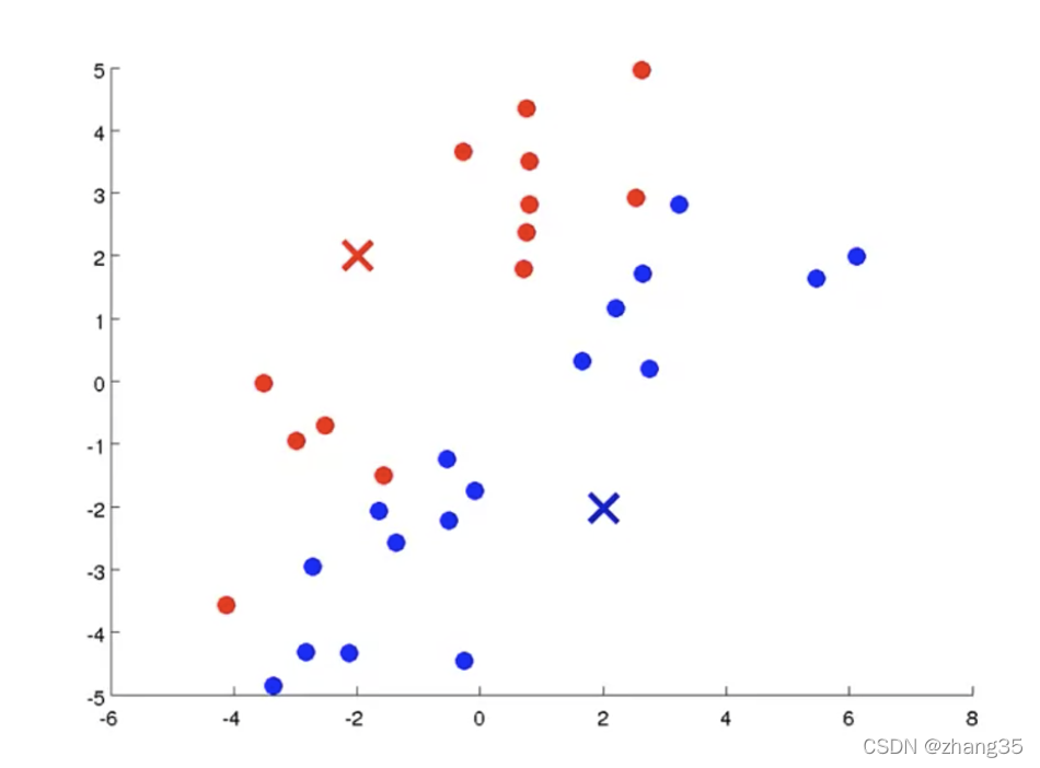
K-Means算法
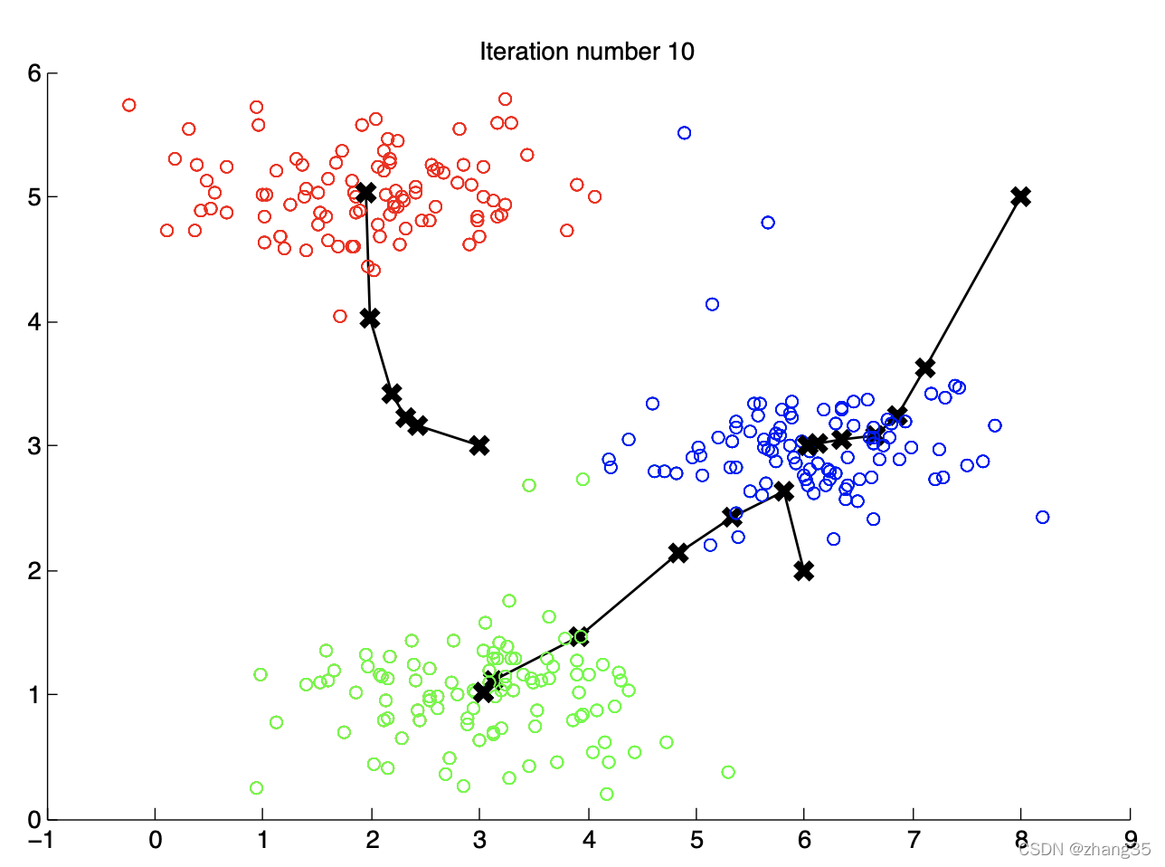
随机找K个中心点(红×和蓝×),将样本标记为最近的中心点:
计算每个类别里样本的平均值(mean),作为新的中心点:
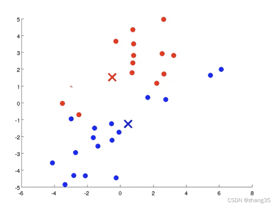
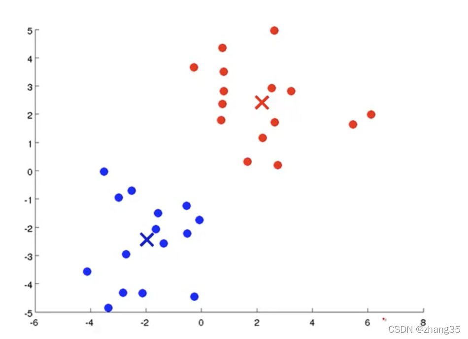
循环执行上面两个步骤,直到中心点不再变化,得到聚类结果:
算法伪代码如下:
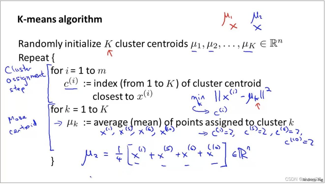
注意:有可能出现某个类别中没有点的情况,这时通常就删掉这个中心点,就变成了k-1个类别。(如果还是需要k个类别,可以再重新随机出一个中心点)
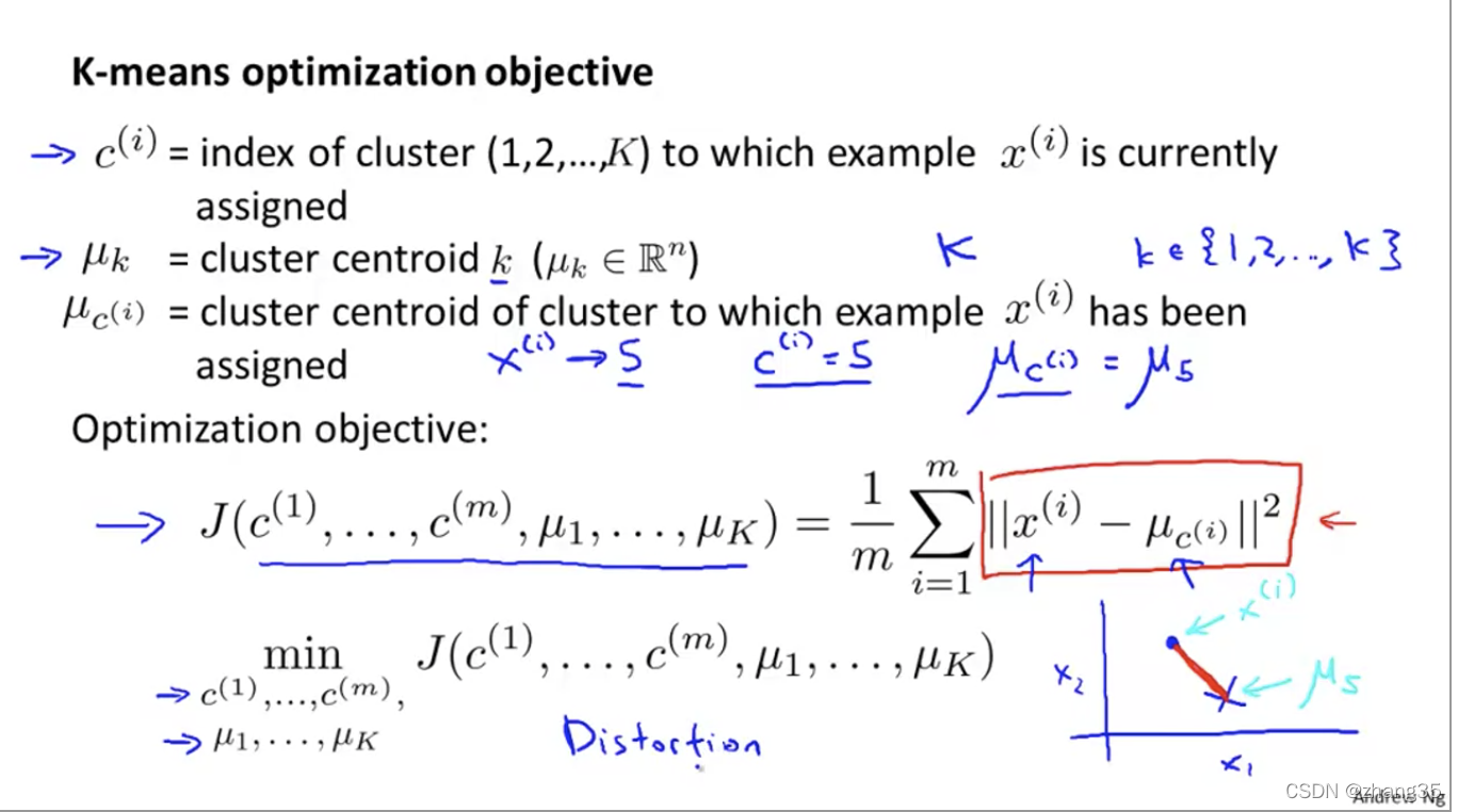
K-means优化目标
这里的J也被称为Distortion函数。
目标就是找出一组中心点μ,对样本标记后得到c,使得J(c, μ) = 样本点到相应标记点的总距离平均值最小:
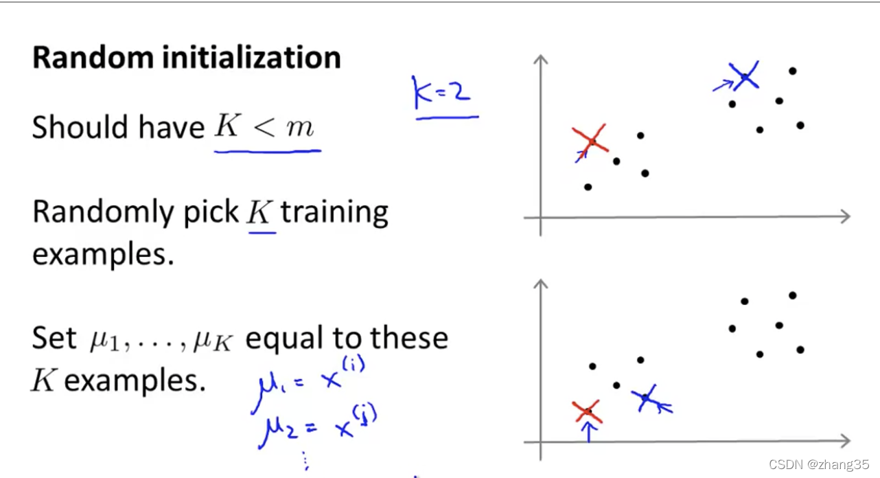
随机初始化
随机从样本点里找K个点,作为初始中心点:
随机选点的不同,K-means的结果也可能不同。右上是全局最优,右下两个都是局部最优:
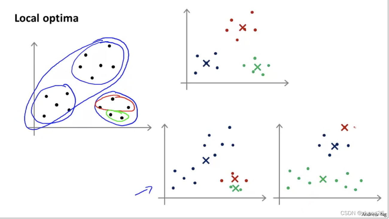
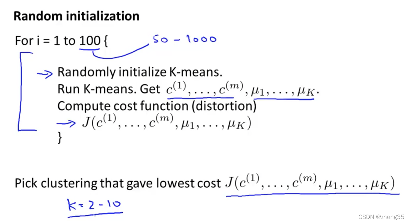
为了保证效果,需要执行多次K-means,尝试多次随机选点,选出代价函数最低的。一般是50-1000次。
当k较小时,比如k=2-10时,执行多次K-means有明显效果。但当k较大时,比如k=100,多次执行可能效果也不会提高太多:
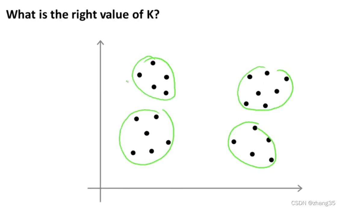
怎么选K
手动选择
一般是靠数据可视化,或者看数据特点,人工选择的。
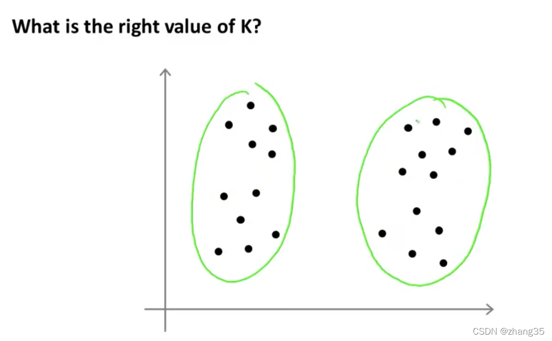
比如下面的样本,选择K=4或K=2都是可以的:
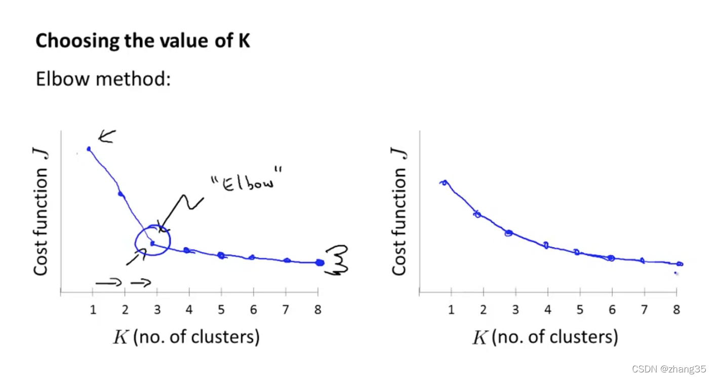
自动选择
左图,Elbow方法:随着K的变化,找到代价函数下降速率的拐点(像肘一样)。
但实际上,有可能出现右图的形状,很难区分哪个是拐点。
所以Elbow方法仅是值得一试,不要抱太大期望。
降维(dimensionality reduction)
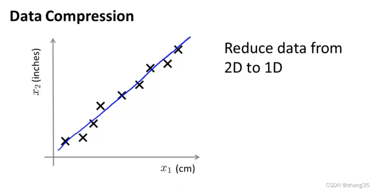
数据压缩
能减少空间占用,也能加速机器学习算法。
当你有成百上千个特征时,需要去下重,即缩减高度相关的。
如下cm和inch的特征(由于有四舍五入的误差,二者并没有完美拟合在一条直线上)。
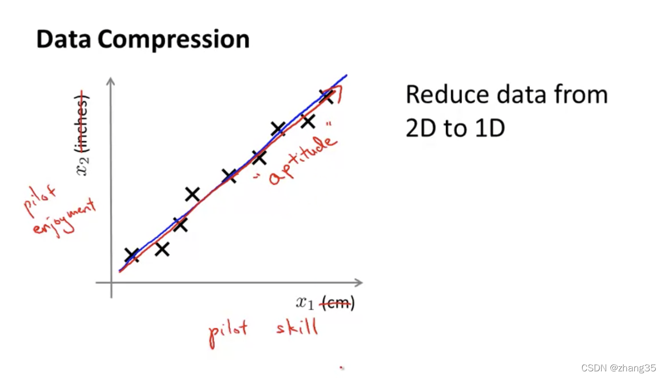
另一个例子,将飞行员的“技巧”和“兴趣”,缩减为“态度”:
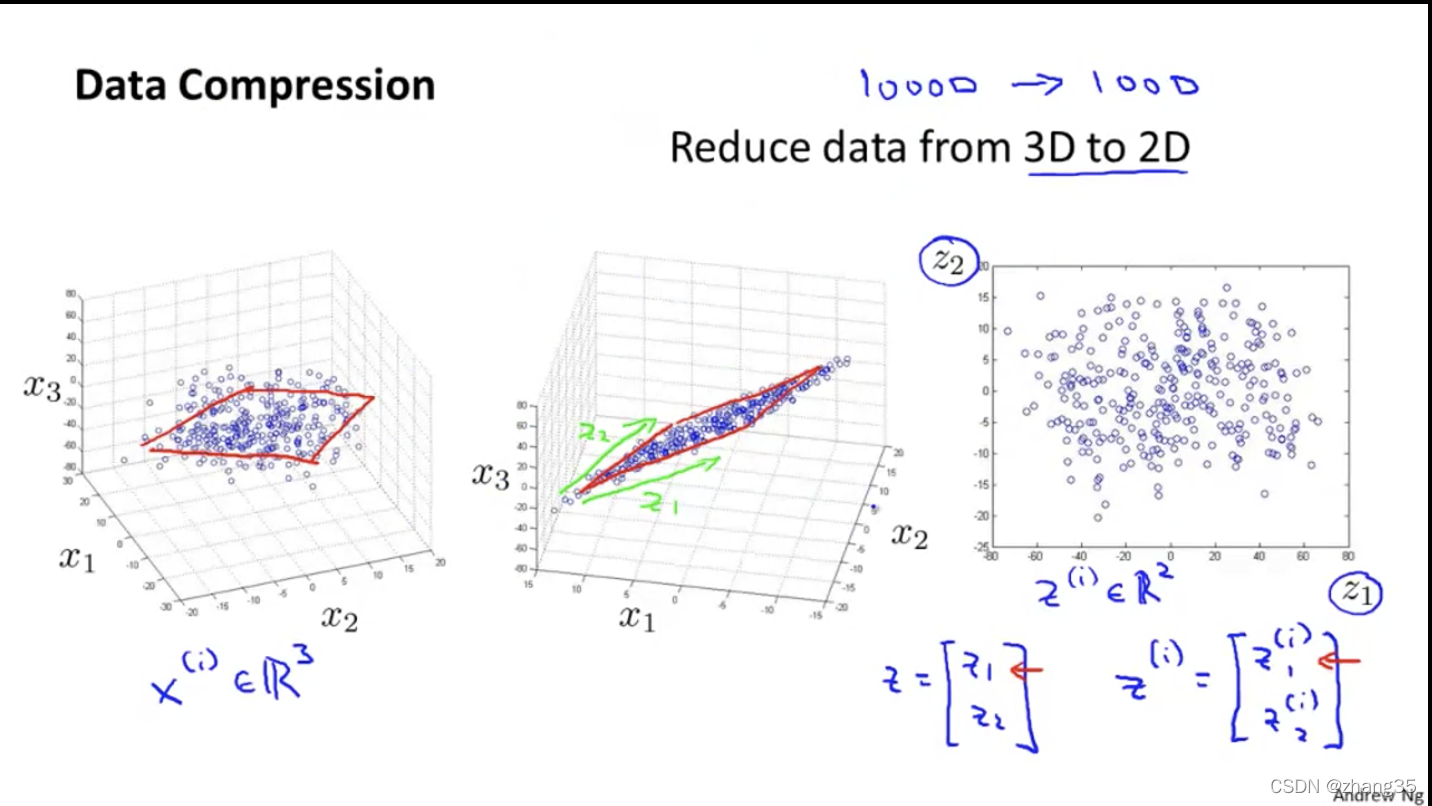
三维降成二维的例子:
数据可视化
因为人类只能看到三维以内的图像,所以为了可视化数据,需要将特征降维到2个以内。
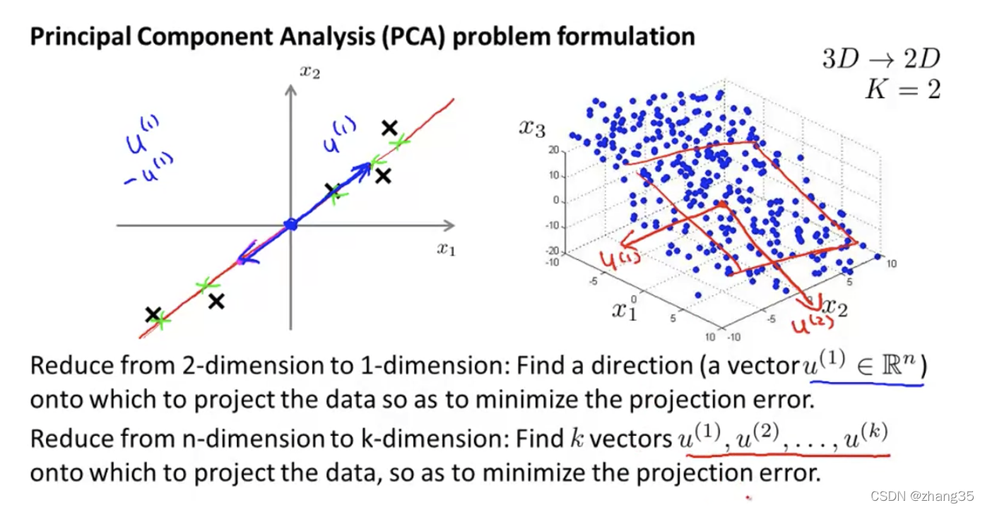
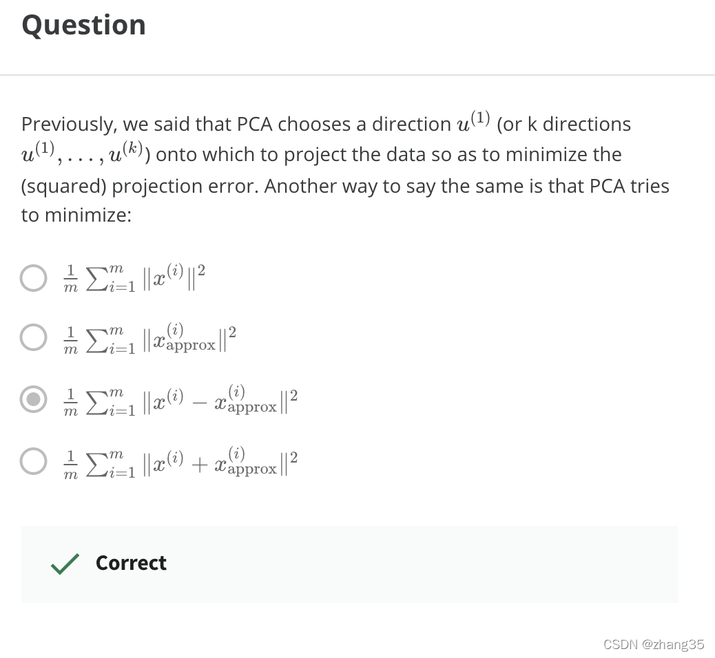
PCA(Principal Component Analysis)主成分分析方法
降维映射后,距离最短的。
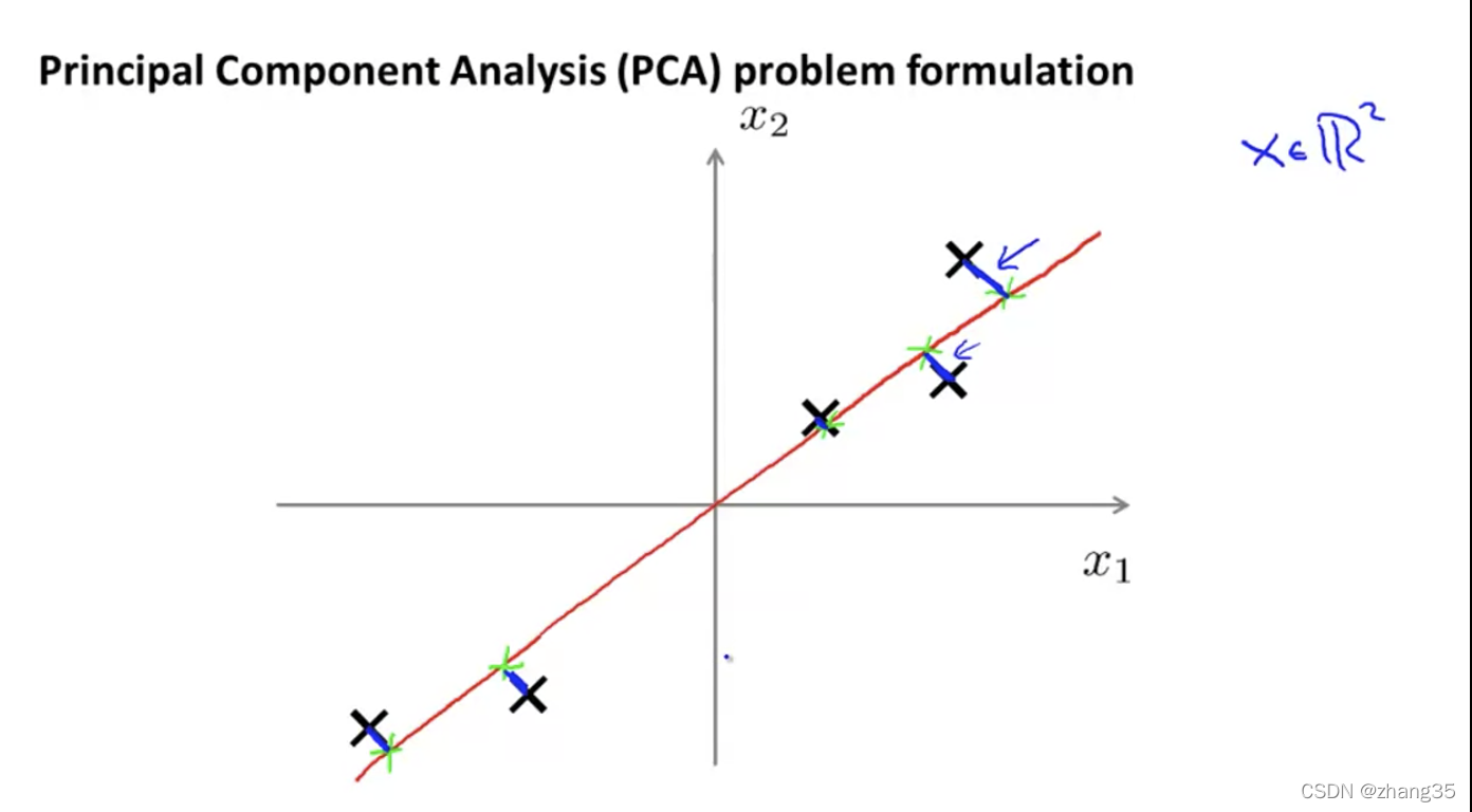
从n维降到k维:找k个向量,使数据映射到k个向量上时,映射距离最小。
数据预处理
使用PCA算法前,要做特征缩放、归一化等处理:

PCA算法流程
名词解释:
eigenvectors 特征向量
eigenvalues 特征值
- 计算协方差矩阵sigma
- 使用sigma作为输入,调用函数svd(sigma)计算出eigenvectors(特征向量),[U, S, V]
- 得到的U是n * n矩阵,取前k列,得到Ureduce ,n * k 矩阵
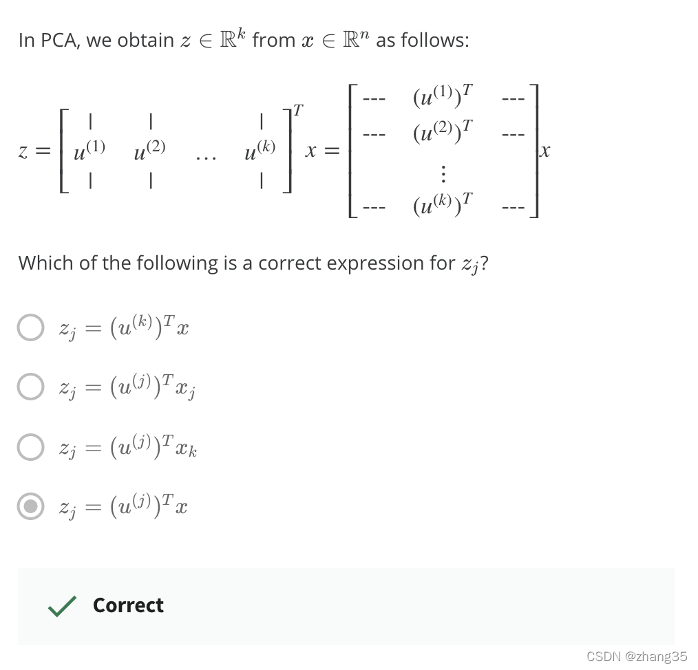
- 得到新的特征:z = Ureduce’ * x

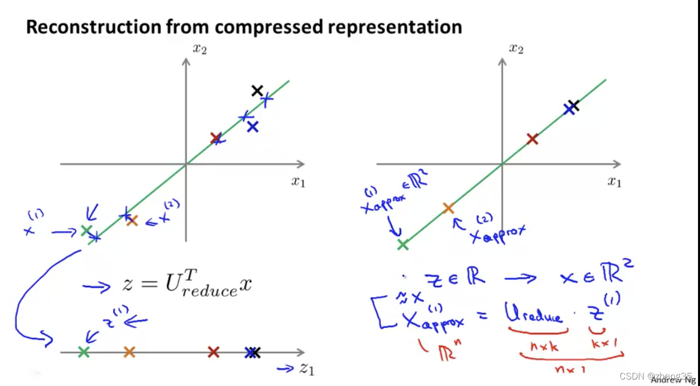
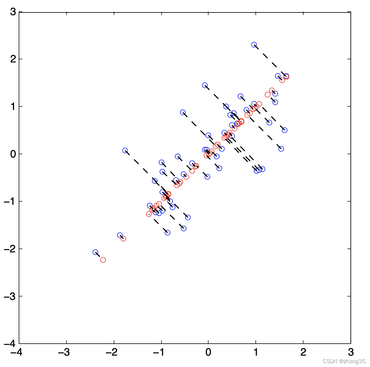
从降维还原数据
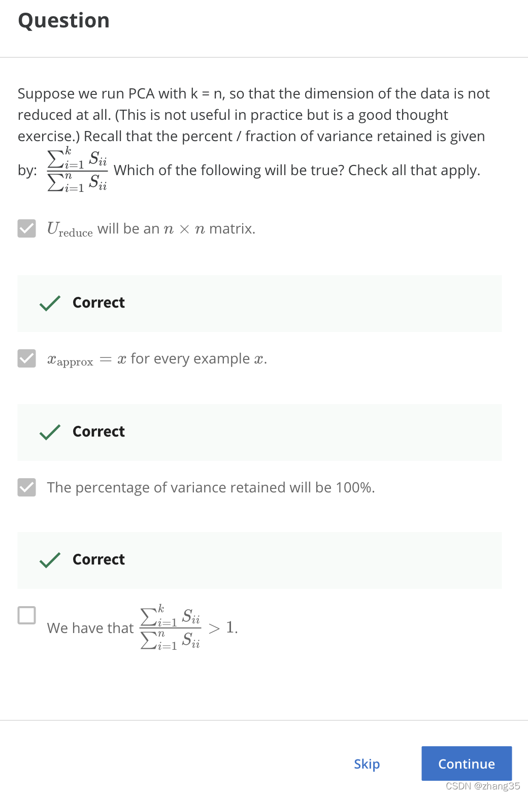
如何选择PCA算法中的k(主成分个数)
Total variation:就是数据离0的距离。
保留足够高的差异度,一般设为99%。
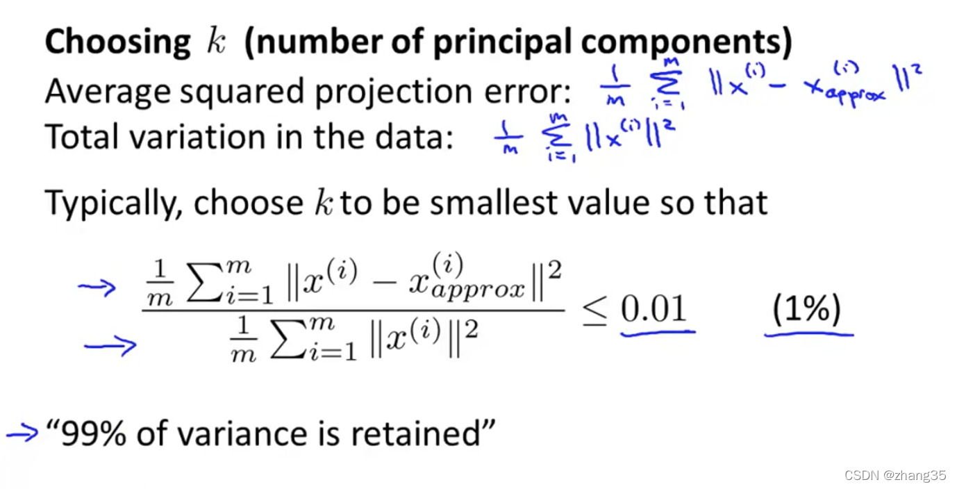
左图,从1开始遍历k,找到第一个符合差异度保留99%以上的k。右图,可以根据[U, S, V] = svd(Sigma)中的S快速计算差异保留度:

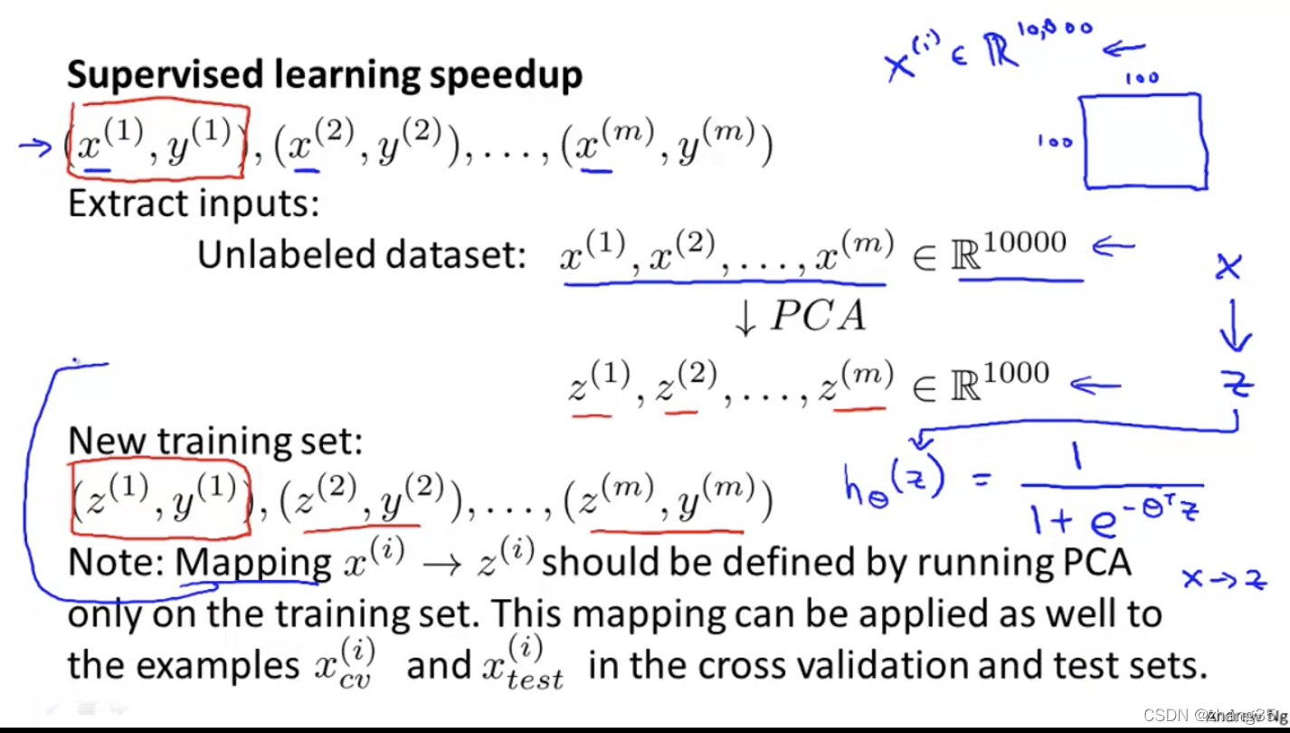
PCA如何加速机器学习算法
将样本的维度从n缩减到k。
注意:只在训练集上运行PCA,找到x->z的映射方法。以后这个映射方法可以再应用到交叉验证集和测试集。
PCA的运用
正确运用:1. 数据压缩 2. 可视化
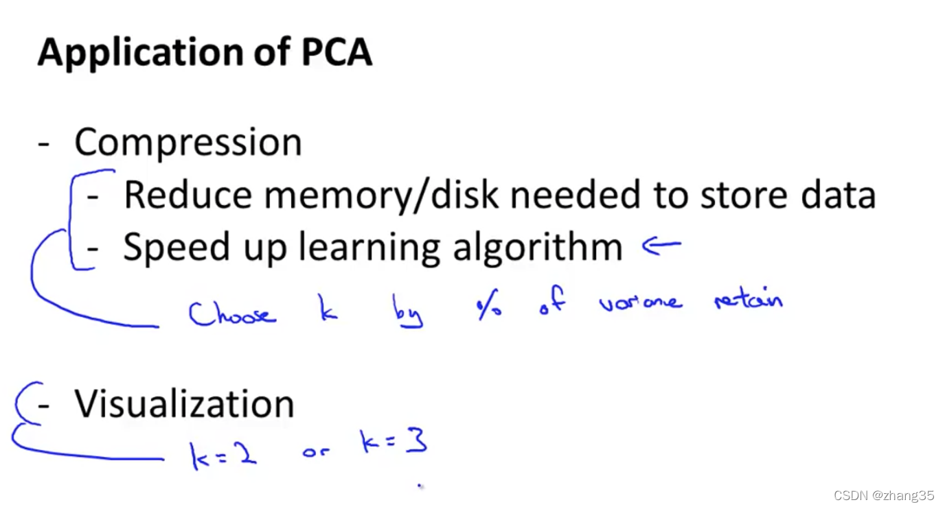
错误运用:缩减特征来避免过拟合
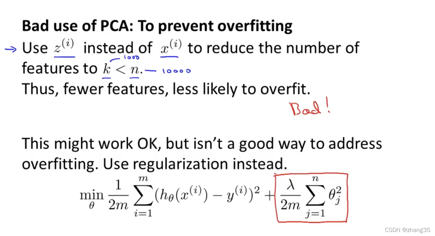
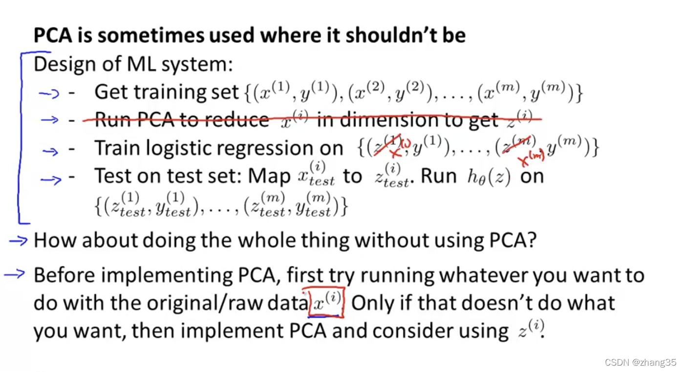
不要上来就用PCA,首先要想不用PCA怎么样?
当内存或硬盘空间不足、算法运行速度过慢时,再考虑加入PCA。
作业
findClosestCentroids.m
function idx = findClosestCentroids(X, centroids)
%FINDCLOSESTCENTROIDS computes the centroid memberships for every example
%   idx = FINDCLOSESTCENTROIDS (X, centroids) returns the closest centroids
%   in idx for a dataset X where each row is a single example. idx = m x 1
%   vector of centroid assignments (i.e. each entry in range [1..K])
%

% Set K
K = size(centroids, 1);

% You need to return the following variables correctly.
idx = zeros(size(X,1), 1);

% ====================== YOUR CODE HERE ======================
% Instructions: Go over every example, find its closest centroid, and store
%               the index inside idx at the appropriate location.
%               Concretely, idx(i) should contain the index of the centroid
%               closest to example i. Hence, it should be a value in the
%               range 1..K
%
% Note: You can use a for-loop over the examples to compute this.
%
m = size(X,1);
for i = 1:m,
    minDist = inf;
    for k = 1:K,
        diff = X(i,:)-centroids(k,:);
        dist = diff * diff';
        if dist < minDist,
            idx(i) = k;
            minDist = dist;
        end
    end
end


% =============================================================

end
computeCentroids.m
function centroids = computeCentroids(X, idx, K)
%COMPUTECENTROIDS returns the new centroids by computing the means of the
%data points assigned to each centroid.
%   centroids = COMPUTECENTROIDS(X, idx, K) returns the new centroids by
%   computing the means of the data points assigned to each centroid. It is
%   given a dataset X where each row is a single data point, a vector
%   idx of centroid assignments (i.e. each entry in range [1..K]) for each
%   example, and K, the number of centroids. You should return a matrix
%   centroids, where each row of centroids is the mean of the data points
%   assigned to it.
%

% Useful variables
[m n] = size(X);

% You need to return the following variables correctly.
centroids = zeros(K, n);


% ====================== YOUR CODE HERE ======================
% Instructions: Go over every centroid and compute mean of all points that
%               belong to it. Concretely, the row vector centroids(i, :)
%               should contain the mean of the data points assigned to
%               centroid i.
%
% Note: You can use a for-loop over the centroids to compute this.
%

for i = 1:K,
    centroids(i,:) = mean(X(idx == i, :));
end


% =============================================================


end
pca.m
function [U, S] = pca(X)
%PCA Run principal component analysis on the dataset X
%   [U, S, X] = pca(X) computes eigenvectors of the covariance matrix of X
%   Returns the eigenvectors U, the eigenvalues (on diagonal) in S
%

% Useful values
[m, n] = size(X);

% You need to return the following variables correctly.
U = zeros(n);
S = zeros(n);

% ====================== YOUR CODE HERE ======================
% Instructions: You should first compute the covariance matrix. Then, you
%               should use the "svd" function to compute the eigenvectors
%               and eigenvalues of the covariance matrix.
%
% Note: When computing the covariance matrix, remember to divide by m (the
%       number of examples).
%
Sigma = X' * X ./ m;
[U, S, ~] = svd(Sigma);


% =========================================================================

end
projectData.m
function Z = projectData(X, U, K)
%PROJECTDATA Computes the reduced data representation when projecting only
%on to the top k eigenvectors
%   Z = projectData(X, U, K) computes the projection of
%   the normalized inputs X into the reduced dimensional space spanned by
%   the first K columns of U. It returns the projected examples in Z.
%

% You need to return the following variables correctly.
Z = zeros(size(X, 1), K);

% ====================== YOUR CODE HERE ======================
% Instructions: Compute the projection of the data using only the top K
%               eigenvectors in U (first K columns).
%               For the i-th example X(i,:), the projection on to the k-th
%               eigenvector is given as follows:
%                    x = X(i, :)';
%                    projection_k = x' * U(:, k);
%
Z = X * U(:, 1:K);


% =============================================================

end
recoverData.m
function X_rec = recoverData(Z, U, K)
%RECOVERDATA Recovers an approximation of the original data when using the
%projected data
%   X_rec = RECOVERDATA(Z, U, K) recovers an approximation the
%   original data that has been reduced to K dimensions. It returns the
%   approximate reconstruction in X_rec.
%

% You need to return the following variables correctly.
X_rec = zeros(size(Z, 1), size(U, 1));

% ====================== YOUR CODE HERE ======================
% Instructions: Compute the approximation of the data by projecting back
%               onto the original space using the top K eigenvectors in U.
%
%               For the i-th example Z(i,:), the (approximate)
%               recovered data for dimension j is given as follows:
%                    v = Z(i, :)';
%                    recovered_j = v' * U(j, 1:K)';
%
%               Notice that U(j, 1:K) is a row vector.
%
X_rec = Z * U(:, 1:K)';


% =============================================================

end
k-means:
pca映射效果:


![leetcode[1706]球会落何处 python3实现(dfs,官方题解for else语法)](/images/no-images.jpg)